
When exploring the foundational mechanics of early computing systems, understanding how first-generation computers handled memory calculation reveals both ingenuity and limitation. These pioneering machines, developed between 1940 and 1956, relied on vacuum tube technology and physical memory systems that laid the groundwork for modern computing architectures.
The Birth of Digital Memory
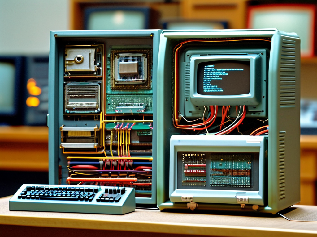
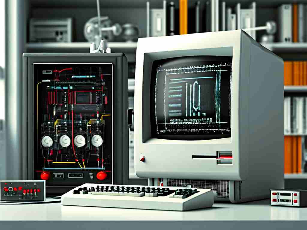
First-generation computers like the ENIAC and UNIVAC utilized mercury delay line memory and cathode-ray tube (CRT) storage. Mercury delay lines functioned by sending electrical pulses through liquid mercury, where the speed of sound in the medium created measurable delays. This allowed data to be stored as sequences of acoustic waves. For instance, the UNIVAC’s memory system could store up to 1,000 words using this method, with each "word" representing a 12-character unit.
CRT-based memory, known as Williams-Kilburn tubes, used phosphorescent screens to store binary data. Electrons would "write" charges onto the screen, creating visible dots that could be read by secondary electron detectors. While innovative, these systems were volatile, requiring constant power to maintain data integrity.
Calculating Memory Capacity
Memory calculation in these systems was fundamentally tied to their physical components. Engineers measured capacity in terms of physical space and component density. For example, the ENIAC’s 20 accumulators could store 10-digit decimal numbers, but its "memory" was functionally separate from its processing units. Programmers manually configured switches and cables to allocate memory for specific tasks, a process that could take days.
The concept of "addressable memory" emerged later, but first-gen systems often used fixed memory blocks. A programmer might reserve a specific delay line or CRT sector for storing intermediate results during calculations. This approach required meticulous planning, as overwriting data mid-calculation could crash the entire system.
Challenges in Memory Management
Physical limitations dominated memory operations. Vacuum tubes generated immense heat, causing frequent hardware failures. The EDVAC computer, completed in 1949, introduced mercury delay lines with a total capacity of 1,024 words—a breakthrough at the time. However, accessing stored data involved waiting for the acoustic pulse to cycle through the delay line, resulting in access times of up to 500 microseconds.
Programmers also faced challenges in optimizing memory usage. Without compilers or high-level languages, they wrote machine code directly, specifying memory addresses in hexadecimal format. A typical instruction might look like:
LOAD A, 0x1F4  // Load data from memory address 500
ADD B, 0x258   // Add value from address 600
This manual addressing left little room for error, as a single miswritten address could corrupt critical data.
Legacy and Transition
Despite their constraints, first-gen memory systems established key principles still relevant today. The separation of storage and processing units evolved into the von Neumann architecture, while the pursuit of higher memory density directly influenced magnetic core memory in second-generation computers.
By 1956, IBM’s 305 RAMAC demonstrated the first disk storage system, offering 5 MB of capacity—a staggering improvement over delay lines. This transition marked the end of the first generation but validated its experimental approaches.
First-generation computers calculated memory through a blend of physics and engineering creativity. Their rudimentary systems, though eclipsed by modern standards, solved unprecedented challenges in data storage and retrieval. Studying these machines reminds us that today’s terabyte-scale memory evolved from engineers manipulating sound waves in mercury and electrons on phosphor screens—a testament to iterative innovation in computing history.